The Physics of Parabolic Microphones: Frequency Dependence of Gain

Introduction

Parabolic microphones are known for their extreme sensitivity, and the origin of their acuity isn’t difficult to guess. It is the most obvious thing about them, which can also make them a liability for field use, namely, their considerable size. Just as a large amount of weak light is captured by a telescope’s parabolic mirror and made amenable to viewing with the much smaller human eye, so too are faint sounds harvested with a reflecting dish that far exceeds the dimensions of our native auditory tools. In both cases, it is a matter of intercepting more of the signal and bringing it to a focus, and the same basic wave physics is at play.

A good overview of the early adoption of parabolic microphones for the field recording of bird sounds was provided by Wahlström (Wahlström, Sten. “The Parabolic Reflector as an Acoustical Amplifier.” Journal of The Audio Engineering Society 33 (1985): 418-429). He describes how Peter Paul Kellog and others first used a 32-inch dish to capture avian vocalizations, with a Yellow-breasted Chat having the honor to be the first species recorded with their novel device.

That a large dish may be cumbersome to transport and use in the field isn’t the only caveat. Users of parabolic microphones soon learn that these devices have a bias that favors high frequencies. Where this is most evident is in the “tinny” quality to the captured sound, which some listeners find off-putting. Others find this drawback significantly outweighed by the benefits of hearing otherwise inaudible sounds, and the boost in signal strength that comes with the high directionality.

The flip-side is that the performance drops off for low frequencies, with a cut-off point below which no benefit is derived. That is, the microphone will capture the same signal power whether the dish is present or not, which may seem curious. This cutoff frequency is given by

$f_{cutoff}=V/a$ ,

where V is the velocity of sound and a is the diameter of the dish. For a=32 inches, this works out to roughly 421 Hz. Most bird vocalizations lie well above this frequency, but we can easily calculate how this limitation will pour cold water on any hopes of wielding small, unobtrusive dishes. An 8-inch parabolic, for example, would provide no gain below 1,500 kHz. The low hooting call of a Mourning Dove would not be be amplified by such a device.

The bias favoring higher pitches can be captured by an expression for the gain as a function of the relative change in frequency. In comparing performance at a frequency f versus a reference frequency f₀ , the gain G as measured in dB is:

$G = 20 \log (f/f_0)$ .

For a change of one octave, that is, for a doubling in frequency, we have the log of 2, which is 0.3, and so the gain will be 6 dB per octave (provided that f₀ is above the cutoff frequency). To put this into perspective, a 10 dB change corresponds to a doubling of perceived loudness. A 6dB change therefore will certainly produce a noticeable difference.

The gain rule is easy to keep in mind, and so is the cutoff condition. Because a wave’s frequency is its velocity divided by wavelength $\lambda$ , the cutoff condition corresponds to a wavelength equal to the dish aperture a. Therefore we can simply say that parabolic dishes provide gain when the waves are small enough to “fit” within the diameter; that is, when $\lambda < a$ . But these handy relationships alone don’t explain why the relative scale of wavelength to aperture is so important.

The Wahlström paper provides a detailed derivation of the gain formula, but the technical approach employed is not trivial. It involves calculating the effect of the dish by means of finding the air velocity at every point in space that results from an incoming sound wave reflected from the surface This is done by determination of a velocity potential, and if that does not sound particularly amenable to an intuitive understanding, it’s because it isn’t.

The goal here is to develop a good physical sense for the frequency-dependent performance of parabolic microphones, using a four-part approach. First, we’ll look at how and why reflections from a parabolic surface converge to a central focal point. Second, we’ll consider the reciprocity property of waves, which allows us to consider the physics both forwards and backwards in time, and to reverse the roles of sources and receivers. Third, we’ll review the concepts of interference and diffraction, as well as Huygen’s wavelet model, which are essential to understanding wave phenomena. Fourth, we will combine our insights in order to derive the 6 dB/octave result, as well as the loss of gain below the cutoff frequency.

If you don’t want to go through the details, here is the ultra-condensed, yet non-trivial explanation:

The Short Version

For all of the energy incident upon a parabolic dish to be reflected to the focal point where the microphone element resides, the wavefronts must arrive moving parallel to the central axis of the dish. When plane audio waves from a distant source enter a dish having some aperture, there will be some unavoidable amount of diffraction, which will cause the wavefronts to no longer be planar. To the degree that they are diffracted, they will no longer reach the surface parallel to the axis. The reflected waves will not be uniformly directed at the microphone element, and there will be a loss in gain. The amount of diffraction is governed by the relative sizes of the aperture and the wavelength. When the aperture is much larger than the wavelength, less diffraction occurs, so the gain remains high. (See figure 15 below for a simulation.) When the aperture is smaller than the wavelength, the diffraction effects render the dish useless. (See figure 16.) In between these extremes, the effect varies as the square of the ratio of aperture-to-wavelength. Gain therefore is larger for short wavelengths, which correspond to higher frequencies.

The Focusing Capability of a Parabolic Dish

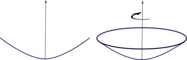
A three-dimensional parabolic dish is a paraboloid, formed by taking a two-dimensional parabola and spinning it around its central axis, as shown in figure 1. A happy result of this relationship is that we can, with no loss in generality, use the simpler case of two-dimensional waves, surfaces, and reflections in order to construct diagrams and visualize wave motion throughout much of this article.

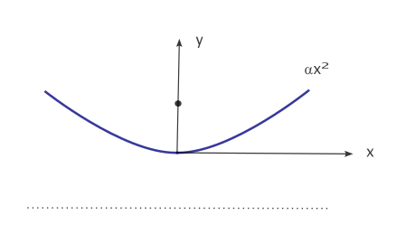
Parabola-Parabolic-Dish — Figure 1. A two-dimensional parabolic curve, on the left, is symmetrical about a central axis. If we were to spin this curve around that axis, it would sweep out a three-dimensional paraboloid shape, which is the form used by telescope mirrors and parabolic dishes.

A parabola can be defined as a curve which everywhere is equally distant from both a fixed point in a space (the focus) and a straight line that does not pass through that point (the directrix). More usefully, if we pick an appropriate coordinate system, the parabola can be expressed according to $y = \alpha x^2$ where $\alpha$ is a constant, as illustrated in figure 2.

Figure 2. Every point on a parabola is equally distant from the focus (the circle on the y-axis) and the directrix (the dashed line at the bottom). It is also described by squaring the x-coordinate and multiplying by a constant, $\alpha$ , in order to calculate the y-value.

Figure 2. Every point on a parabola is equally distant from the focus (the circle on the y-axis) and the directrix (the dashed line at the bottom). It is also described by squaring the x-coordinate and multiplying by a constant, $\alpha$ , in order to calculate the y-value.

There are two properties of a parabolic surface that will make it particularly useful. The first is that it reflects all trajectories parallel to the y-axis to the same focal point. Imagine that someone had constructed an unusual pool table in which one side took on a parabolic shape, as shown in figure 3(a). Balls which were aimed along parallel lines, as shown, would always rebound off the surface so as to cross the same focal point F, regardless of where they were shot from. This is the case because the angle at which the ball bounces off the table must be equal to the angle at which it strikes, as shown in diagram (b). This angle is measured relative to the line that is perpendicular to the surface, and because the surface has a gentle curve, the perpendicular, or normal line, is different at each point on the wall. It is the unique parabolic shape that ensures that the surface orientation will always lead to reflection back to the focal point.

Figure 3. (a) Billiard balls rebounding from a parabolic wall, seen from above. All paths parallel to the y-axis will lead to rebounding balls crossing the same focal point. (b) The changing curved shape of the parabola means that the perpendicular direction (dashed line) is always oriented to direct the reflection to the focal point. The angles of incidence and reflection are always the same; the perpendicular lies midway between the two directions of motion.

The second key property has to do with the distance travelled. For each of the starting positions shown in figure 3 (a), the total distance each ball will traveled in order to reach the focus will be the same. This is important for plane waves (rather than projectiles) impinging upon a parabolic surface, because it means we will not have any destructive interference effects between waves that arrive at the focus. We will say more on interference effects shortly. Brief derivations of these two properties are given in the appendix at the end of this post.

Reciprocity

It is clear that for the scenario in figure 3(a), where a billiard ball strikes some point on the parabolic wall and rebounds to cross the focal point F, that we could run the scenario backwards and observe something quite similar. That is, if we shot the ball from the focal point back at the same location on the curve, it would move off along the original incoming path. This symmetry is the basis of reciprocity, the fact that we can run the process “backwards” and well as “forwards” and effectively change nothing but the ordering with respect to time. (We are of course ignoring frictional effects which cause the ball to slow down and which would make it clear if we were playing a film of the motion backwards.)

Let’s now consider the case that the parabolic surface has been made into a mirror, and instead of billiard balls we direct a narrow beam of light into it. (We must point out something we will return to later, and that is that the wavelength of visible light is far smaller than the dimensions of any practically-sized mirror.) We can even keep our pool table model, with the parabolic side now made of polished silver, and a handheld laser placed at various positions instead of billiard balls. Provided that the laser is always oriented parallel, we now have the case of incoming rays that must all cross at the point marked F.

A three-dimensional, paraboloid version of this is what lies at the heart of the reflecting telescope invented by Sir Isaac Newton. Roughly speaking, such a telescope harvests a wide cross-section of light and brings it to a focus by using a parabolic mirror. The light is then diverted from the focal point to a place where an image can be formed for viewing. The principle of reciprocity points to a another way to use such a mirror: suppose we place a small lightbulb source at the focal point. The light will be reflected back out into a collection of parallel rays, forming a collimated beam. Such is the design employed by searchlights, flashlights, and headlights, which are effectively Newtonian telescopes run in reverse.

As long as we take some care, reciprocity can also be applied in regards to properties that we can quantify, such as power (the rate at which energy is transferred). Here it is useful to consider another wave scenario, the expanding circular waves on a still body of water that results from, say, a pebble being tossed in. We will simplify this by representing the train of waves as a single “pulse” expanding outwards, and we’ll also imagine the water is in a perfectly circular pool with the pebble striking in the exact center. Although the pulse consists of a vertical displacement of the water’s height, making it a three-dimensional phenomena, the wave itself moves in just two-dimensions.

Figure 4 shows the expanding wavefront which, upon meeting the circular boundary, must be reflected back. Just as with the case of the billiard balls, we are neglecting any kind of dissipative effects that would rob energy from the waves. In that case, the inward motion is the time-reversal of the expansion, and upon seeing a video it would be impossible to deduct which was the forward or reverse. Suppose the initial power at which the wave leaves the center is P₀ . When it reaches the periphery, this power will be uniformly distributed along the entire wall. We can imagine this wall divided into N identical sections. Each would receive an incoming power of P₀ /N, which it then re-radiates back towards the center.

Figure 4. The expanding wavefront for a single pulse which leaves a central point, reflects upon a wall, and converges back. The total power at any time is P₀ , but because the wave occupies a different amount of space at different times, we must be careful in tracking how much power arrives at any given point.

The important takeaway from this is that we need to be cognizant of the way in which waves spread out whenever we talk about the power associated with them. We don’t need to worry about this for billiard balls or other projectiles because they are localized and always occupy the same amount of space. This may all seem trivial, and in a sense it is, but it will be important at a later point.

Interference, Wavelets, and Diffraction

We’ll now shift gears and review some critical properties of waves, starting with interference, which is a consequence of the fact that waves add together. More formally, we say that they obey linear superposition, so that the total amplitude (such as the height of a water wave) that results when several waves are present at the same place is simply the sum of the individual amplitudes. Consider figure 5, where a duck floats on an otherwise still lake (a), until the wake from a distant speedboat arrives. The duck will be momentarily lifted (b) some vertical distance (the amplitude A) by this transient disturbance. Had an identical boat passed in an identical manner on the other side (c), with two waves arriving simultaneously, the duck would be lifted to twice that height (d), or an amplitude 2A. This is an example of constructive interference.

Figure 5. (a) The wake from a distant speedboat moves across a still lake, towards a duck. (b) As the wave passes the duck is lifted momentarily to a height equal to the amplitude A. In the case of two waves (c) coming from opposite sides, the duck will be lifted to twice the amplitude (d) when they meet, due to constructive interference.

More generally, for waves which feature alternating troughs as well as crests, the situation will be more complex. But the idea at the heart of it remains simple: as several waves arrive at the same spot, their amplitudes add together at that moment. Figure 6 shows an example where two nearby source on the left side create waves which are perfectly out-of-phase. As the waves move to the right, they spread out and overlap one another along a line between them. This is visible as a light blue region in which the color never changes; here, destructive interference occurs, leaving nothing, nether a net positive nor negative amplitude.

Figure 6. Two sources on the left side, one above the other, emit right-traveling waves which are opposite in phase, as represented by the colors. As they move to the right they spread out and overlap to some extent, and in this region they cancel due to destructive interference, leaving a band where no waves occur.

We will next employ superposition in a novel way. First consider the wave disturbance created by a “point” source, such as what occurs when a small pebble is tossed into a still pond. A circular wavefront will expand from this point, moving with the same speed in every direction. But consider what would happen if a series of such expanding rings were made by identical point sources spaced out in a line, as shown in figure 7. We see that after some time that the leading edge (on the right) of the collection of each of these circular “wavelets” forms an advancing straight line, That is, a plane wave, like the line of surf coming in the the beach.

Huygens-wavelet — Figure 7. Five point sources on the left side creating expanding wavelets. The leading edge of these combined wavelets soon becomes the straight edge of an advancing plane wave.

The motion of any wave, no matter how simple or complex, can always be determined by treating it in terms of the superposition of circular wavelets expanding from a collection of point sources. This insight, due to Christian Huygens (1629 –1695), is invaluable for understanding what these waves will do upon meeting an obstacle or passing through an aperture. In the latter case, which is important for us, there is only a limited source of expanding wavelets, and this can lead to some surprising results as these wavelets spread out and interfere with one another. These are diffraction events.

The classic way to introduce diffraction is to imagine plane waves moving from left to right, that are incident upon a barrier that contains an aperture, as shown in figure 8. What we find on the right side of the barrier will depend on the relative size of the wavelength and the aperture.

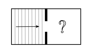
Figure 8. Plane waves moving from left to right are incident on a barrier with an aperture.

Let’s next examine a series of animations that show what happens on the right side of the barrier when plane waves (with various wavelengths) arrive at apertures having different sizes. Then we will use the wavelet model to explain exactly why they look as they do. Figure 9 shows three different results in which plane waves pass through a gap which is: much smaller than the wavelength (left); much larger than the wavelength (middle); and comparable to the wavelength (right). Recall that wavelength is the distance, along the direction of motion, between successive crests (or troughs) of the wave. (Note that in each case the aperture is on the left side and the plane waves arriving there from even further to left are not shown.)

Diffraction-wavelets — Figure 9. Diffraction effects from plane waves passing through an aperture. On the left, the ratio of wavelength to aperture is about 6; in the middle, it is 0.06, and on the right, it is 0.6.

The left diagram is the easiest to understand. Since the aperture is very small, about six times smaller than the wavelength, it is effectively no different from a point source itself, so the emerging wave fronts expand in a circular manner. In the middle diagram we have gone to the other extreme, where the gap is so large (about 16 times the wavelength) that it permits a great number of wavelet sources, resulting in (approximately) plane waves passing through. On the right, we have something intermediate, with some subtle features which we don’t see in the other cases. These are destructive interference effects, similar to what was seen in figure 6; they appear as “rays” in which the color does not change. We can explore effects like these in greater detail by using some careful geometrical constructions as follows.

In figure 10 (a) we consider the behavior of waves emerging from the gap as seen from the point marked O. It will simplify matters if we take this point to lie very far from the gap, so that R is much larger than a, where R is the distance and a is the width of aperture.

Figure 10. Definition of an observation point O, far from an aperture of width a that will act as a source of waves. Of particular importance is the right triangle with the short side y and long side R. This distance R is taken to be much larger than the aperture a.

The total amplitude that will be seen at point O will be the sum of the amplitudes arriving from each of the wavelets within the aperture. Here we encounter the question of how to divide up the space in the gap so as to model a collection of wavelets. We might first divide it into two parts, and approximate the aperture as having three sources: one in the center and one at each end, as shown in figure 11(a). The shading in the diagram indicates how it has been partitioned. Note the right triangle that describes the distance between the sources and difference in the path length, $\delta$ . This triangle is identical to that formed by the sides x,y, and R in figure 10. That means that the ratios of the lengths must be the same, so we can write $\delta / (a/2) = y / R$ .

Figure 11. Close up of the aperture and how it is analyzed. In (a) we have divided it into two portions, allowing us to treat it as consisting of three wavelet sources marked 1,2, and 3. In (b) we have made four divisions resulting in five sources.

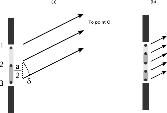
The value of $\delta$ in comparison to the wavelength is the most critical part of this scenario. Consider what would happen if it were equal to one half of the wavelength. The wavelets from point 2 and point 3 would arrive at point O exactly out of phase, as would those from points 1 and 2. Under this condition, there would be total destructive interference at the point O. Because the triangles are similar, then, we know that the y-values at which no power arrives must be given by

$y =(R \lambda /2) / (a/2) =R \lambda/a$ .

But we could have divided the aperture into four zones instead of two, as shown in (b), in which case we’d still get the same end result. This means that the above expression would have been $(R\lambda/2)/(a/4)=2R\lambda/a$ . Or we might have divided into six, or eight, or any even number of parts. We see the trend emerging here: destructive interference will result in a series of locations, given by

$y = m R\lambda/a$ ,

where m= 1,2, (or -1, -2, -3) etc.

This is the explanation for the pattern that is evident in the rightmost animation of figure 9. What appear as motionless bands in this diagram emanating from the aperture are the destructive interference minima corresponding to m=+/-1.

Outside of these minima, that is, towards the top and bottom of the animation, we will have regions where at least some amount of constructive interference occurs. But it is only between the m=-1 and 1 minima, that is, “straight across” from the aperture, in which the wavelets can add together to produce a significant amplitude. This can be seen as a result of the symmetry of the configuration; if y is zero, all of the wavelet sources in the gap lie effectively the same distance from point O, so the results add up constructively. Moving off in either direction must diminish the result until the first set of minima are reached. We can capture this in terms of the power incident on a distant plane, as shown in figure 12.

This diffraction pattern is a key result that can show up with any kind of wave phenomena. Although the interest here is acoustical, it also plays an important role in the determination of resolution for optical instruments (see how it features in the demonstration of aberrations in roof prisms here). A future article will discuss how this pattern is also intimately connected to the Fourier transformation used to generate spectrograms.

We can use these results to help quantify how the wave power is distributed upon exiting an aperture. Consider the left animation from figure 9, where a point-like aperture gives rise to circular wave fronts. We can imagine a small sensor that we could place at the gap in order to measure the total power radiating out, which we denote P₀ . Similar to the case with figure 4, as the wave travels and spreads out, the power will be uniformly distributed across the expanding semicircles (or in 3D, half-spheres) as shown in figure 13 (a). The amount of power that a receiving device would intercept will depend upon what fraction of the total that it can intercept. This will be a function of both the cross-sectional areas of the waves and the area of the listening (receiving) device. The total hemispherical area, at a distance R from the source, will be $2\pi R^2$ , so an antenna or microphone with an effective area of A_rwill collect power at a rate P given by $P = P_0 A_r / 2\pi R^2$ .

Figure 13. (a) A receiving device with effective area *A_r* positioned to detect some fraction of the power from plane waves radiating through an aperture in which the wavelength is large compared to the gap. In (b) the gap is large compare to the wavelength. In this case, the same receiver will intercept a much larger fraction of the total power.

Now consider the other extreme, in which an aperture emits waves with a wavelength that is much smaller than it is, as animated in the center frame of figure 9 and shown here in diagram (b). Although some of the power will be radiated out into the narrow, off-axis bands, it will be less than 10% of the total, and we will neglect it here. We saw from the diffraction pattern image of figure 12 that the bulk of the power is delivered into the region between m= +/-1. What is evident here is that in the case of (b), the receiving device will be intercepting a much larger fraction of the total power emitted by the source than it did in case (a).

We can make a quick estimate of how much more power our device harvests in case (b) as follows: since the distance from the peak to the first minimum is $y=R\lambda/a$ , it covers an area of about $\pi R^2 \lambda^2/a^2$ . In case (a) it was spread out over an area of $2\pi R^2$ (which is also the area the power would be spread across if it were coming from a point source). The ratio of these areas tells us how much more concentrated the power becomes in case (b), and that ratio is proportional to $a^2/\lambda^2$ . This is a key result that underpins the frequency dependence.

The Parabolic Dish as a Radiating (and Receiving) Aperture

We can now bring all of these pieces together in order to quantify the gain of using a parabolic dish.

First suppose that we have a point source radiating at power P₀, and a receiver some distance R away with a cross-sectional area A_r . The total power it will measure is $P = P_0 A_r/4\pi R^2$ , which is the radiating power times the ratio of the dish area to the total radiated area. We will now place the point source at the focus of a parabolic dish having an aperture of width a. Regardless of the wavelength of the radiation, it will strike the dish and reflect to form plane waves within the volume of dish, and then radiate out from the aperture, at which point some degree of diffraction may occur. From the perspective of a receiver anywhere to the right of this radiating dish, the situation looks no different than if we had a flat wall with an aperture of width a being radiated with plane waves on the other side.

The radiating aperture will, depending on its size compared to the wavelength, emit something ranging from hemispherical wavefronts just like those from a point (when the wavelength is larger than the aperture) to tightly focused plane waves which from a beam (in the other extreme of wavelengths very small compared to the aperture). We know that over 90% of the power will be contained within an angle $\theta$ which becomes smaller as the ratio $\lambda /a$ decreases. We can approximate the power at the receiver as $P' = P_0 A_r / \pi R^2 (\lambda^2 / a^2)$ . The addition of the dish results in proportionately more power according to $P'/P \propto a^2/2\lambda^2$ . When speaking of a dish used as a radiating antenna, this ratio is appropriately termed the directivity. Due to reciprocity it is also the gain when the same device is used as a receiver.

We see this by looking at the radiating aperture of the dish and running time backwards, as shown in figure 14 (a) for an intermediate case of diffraction, where the wavelength and aperture are comparable in size. Here we have curved, contracting wavefronts approaching from the right, carrying a total power P₀ , which must, via reciprocity, become plane waves within the dish and then reflect perfectly back to the focal point. The total power collected will be P₀ but only because the incident waves are appropriately curved. In practice, by using the dish as a receiver we will be picking up plane waves, and these must diffract upon entering the dish. As shown in diagram (b), these will undergo the same diffraction and spreading out that emitted waves would take.

Figure 14. (a) Should the appropriate converging wavefronts be incident on an aperture, all of the power will be transferred into plane waves passing to the other side. (b) If the same aperture receives plane waves instead, as is typically the case, they will diffract out upon passing through. According to reciprocity these are effectively the same.

So now the problem is clear: if plane waves enter the dish aperture and undergo diffraction, then some portion of the wavefronts will not arrive “straight on” to the parabolic surface, They will have a smaller angle relative to the local normal direction, and so will not reflect back to the focus but instead to a point further away from the dish. The extent of this misalignment will depend on the relative size of the wavelength to the aperture.

Figure 15 shows what happens to a series of short wavelengths incident upon a wide parabolic surface. There is a small amount of diffraction near the edges, but by the time the entire wavefront has been redirected, we can see that most of the reflection forms concentric circular wavefronts that converge at the focus.

Parabolic-reflection-waves=diffraction-focus — Figure 15. A numerical simulation of a series of short-wavelength plane waves incident on a parabolic surface with a relatively wide aperture. Most of the reflections converge at the focal point, except for those from the extreme sides of the curve, where diffraction has subtly altered the angle of incidence (and hence of reflection).

Figure 16 shows the same simulation, but with a much longer wavelength. Now as the wave is reflected off the periphery it is clear that much of this energy will not be directed to the focal point, but instead is spread out through space along a vertical line through the center. Only a narrow, central portion of the incoming plane wave is reflected back to the focus.

The diffraction caused by entering the aperture of the parabolic dish changes the direction of the wavefronts, leading to reflections which do not converge upon the focal point. This is the key reason why parabolic microphones function as they do.

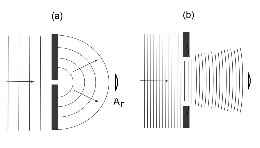
We can also give a simple and beautiful demonstration of why there is no gain when the wavelength is larger than the dish diameter. In figure 17 (a) we have a point source producing a long wavelength, placed at the focus of a dish with a small aperture. In (b) the aperture is increased, but it still stays smaller than the wavelength. In both cases, the power is uniformly radiated to the right in hemispherical wave fronts. It would be impossible to tell, at a distance, just how larger the aperture was. Now consider the reverse, where perfectly hemispherical wave fronts converge on an aperture, which is the only way that it would be able to collect the full incident power. If the waves are arriving in this manner, it would not matter if the large or small dish were employed; they both would still collect all the incident power, as would the point source (now acting as a sensor or microphone element) if it were places at the center of these converging waves. It is a bit like how a funnel will harvest all the water going in no matter how big the “exit” hole is. As long as the wavelength is longer than the aperture is wide, it does not matter how big the dish is; you’ll always collect the same power.

Figure 17. Long wavelengths emitted from a point source inside a parabolic dish with apertures much smaller (a) and (b) smaller than the wavelength. In both cases, the wavefronts expand to the right in uniform semicircles with the same total power. Running these in reverse immediately makes it clear that both dishes, despite their difference in size, would collect the same total power, as would the point source (the microphone element, or sensor) alone.

Plane waves incident upon the dish aperture will diffract to the same degree that they would if they were radiating outward because a point source was placed at the focal point. Some of these diffracted waves will be deviated in their approach and will strike the dish at a shallow angle that will not bring them to a focus, but some portion of the wavefronts will continue straight and strike the dish at the appropriate angle. The fraction that do so by depends on how widely the diffraction spreads out the incoming plane waves. We showed in the context of the dish as a radiator that the fraction of the beam that falls on fixed receiving antenna varies as $a^2/\lambda^2$ . The same must be the case when the dish is a receiver.

Since the wavelength and the frequency f are related to the wave velocity V according to $\lambda = V/f$ , we can then say that the power which can be utilized by the dish must vary as $a^2 f^2$ , and writing in decibel units, the dependence of gain on area and frequency must go as

$G = 10\log(a^2 f^2)$

For a dish with some fixed size, and assuming that the wavelength is less than the diameter, the only dependence is the frequency. The change in gain that occurs from doubling the frequency (that is, by going up by one octave) is given by $10\log(4f_0^2)-10\log(f_0^2) = 10log(4)=6$ . Hence the 6 dB/octave frequency rule.

Readers that are interested in parabolic dish performance will find that the topic gets more attention, as well as a broader range of detail, in the context of antennas for electromagnetic signals. See, for example, Warren Stutzman’s “Estimating Directivity and Gain of Antennas” in Antennas and Propagation Magazine, IEEE. 40. 7 (1998).

Image credit: Amanda Slater, Creative Commons, https://commons.wikimedia.org/wiki/File:Parkes_Radio_Telescope_(CSIRO).jpg

Appendix: Reflection from a Parabolic Surface

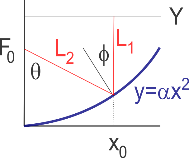
For a parabolic curve expressed by $y=\alpha x^2$ , the slope is given by the first derivative $y' = 2\alpha x$ , and so the slope of the normal line at that point must be $-1/2 \alpha x$ . Now we consider the reflection of an incident ray (in red) as shown in figure A1 below. The term “ray” here means nothing more than a direction of motion, and could describe the path of a projectile or, say, a narrow beam of light. Since the incidence and reflection angles must be the same, we can see that $\theta = 2 \phi$ . For some point x₀ on the curve, we will denote the point F₀ as the point on the y-axis where the reflection crosses, as shown. We then have $\tan \theta = x_0 / (F_0-\alpha x_0^2)$ . We also can use the slope of the normal line to relate to another tangent, namely $\tan \phi = 2\alpha x_0$ . The double angle formula for the tangent,

$\tan 2 \phi = 2 \tan \phi / (1-\tan^2 \phi)$ ,

then gives us

$x_0 / (F_0-\alpha x_0^2) = 4\alpha x_0 / (1-4\alpha^2x_0^2)$ .

Solving this equation yields $F_0 = 1/4\alpha$ independent of x₀. Therefore all incident rays must reflect to the same spot.

Figure A1. Geometry used to derive key reflection properties of a parabolic curve.

Next we consider some vertical height Y above the parabola, and determine the distance to focal point F₀ by way of reflection. The first leg of the journey, which is purely vertical, covers a distance $L_1 = Y-\alpha x_0^2$ . The second leg is given by $L_2=\sqrt{x_0^2+(F_0-\alpha x_0^2)^2}$ . The term in the radical easily works out to $F_0+\alpha x_0^2$ because $F_0=1/4\alpha$ . The total distance is then $L_1+L_2 = Y+F_0$ , which is independent of x₀.

Birding Despite Disability