
The famous Zeiss “paper” by Weruach and Dörband (translation attached below) on the development of phase coatings for roof prisms describes a simple test to determine if an optical instrument has coated prisms or not. They describe the use of two linear polarizers with the device placed in between; with phase coating present, one will observe the maximum transmission of light with the polarizer axes parallel, but if the prism is not coated, more light will pass when the polarizers are “crossed” or perpendicular.
As is the case with anything published by an optics company on the subject of phase coatings, there are no technical details given to go with this, so if you have any interest in why their proposed test works, you’ll have to work through the physics yourself. Or, assuming that doesn’t excite you, you can keep reading, because I’ve done the calculations for both S-P and A-K prism designs. (The Zeiss reference does not go into any detail on how these might differ in their test.) The Python code is at the bottom of this post, and there is some additional discussion at The Physics of Roof Prism and Phase Coatings, Simplified: Polarization Effects.
On the general topic of roof prisms and phase coatings, please see my series of posts:
The Physics of Roof Prisms and Phase Coatings
The Physics of Roof Prisms and Phase Coatings, Simplified: Part I
The Physics of Roof Prisms and Phase Coatings, Simplified: Part II
The Physics of Roof Prisms and Phase Coatings, Simplified: Part III
Technical References for Roof Prism Resolution Loss, Phase Coatings, and Related Topics
Beyond performing the calculation of the output polarization for the two roof prism designs, I wanted to verify the results of the Zeiss polarizer test experimentally. This is easy to do for the case of coated roof prisms; simply use any pair of decent roof bins made in the last 30 years. But unless you are a collector of older models, finding uncoated prisms may take a bit of work, especially if you don’t want to pay a lot of money.
In my quest for uncoated prisms, I started with Edmund Scientific. Yes, they changed their named to Edmund Optics, but I’m using the old name because when I was an astronomy buff as a kid, that is what they were called, and the moniker has sentimental value. I collected their catalogs and knew their inventory inside and out. I even used to own one of their odd-looking yoke-mounted Newtonian reflectors. Digression alert:
Anyway, Edmund today will sell you a new, uncoated, Amici roof prism with an 8mm aperture for only… $87. That seems about a factor of ten too high by my reckoning, so I went searching elsewhere. I did look into some eBay listings for older binoculars, but grew impatient with sellers that could not definitively date the products they were advertising.
Eventually I found this from Ali Express, described as an “Amici Optical Half Roof Ridge Prism” but was actually a Schmidt prism, for about $7. My inquires as to any coatings only produced confusion on their end, so I just ordered it. It arrived several weeks later, and placing it between my laptop LCD screen (a ready source of polarizer light) and a polarizing sheet instantly revealed the color shifting signature of coatings. How annoying.
Next I decided to look for a cheapest monocular available, with the hope that it would have an uncoated prism. On Amazon I discovered something called the “ZEAL’N LIFE 40×60 Monocular Telescope High Power Monocular” (for Adults!) going for $4.99 and free Prime shipping. It arrived within a few days and with great excitement I placed it between screen and polarizer and found… no interference colors! The roof line was clearly evident, but upon rotation, the two halves of the pupil only changed in shades of gray. This was very promising, but I was still uneasy because I did not immediately see any obvious difference in light transmission for the parallel versus crossed polarizer configurations. When I went through more careful measurements, it was in fact observable, but it took some effort to be certain that I was really seeing it.
And this gets to something about the Zeiss reference that is potentially a bit misleading. The difference in light transmission for parallel and crossed polarizers is not dramatic when the prism isn’t coated (but it is when the coating is present). This is borne out by an analysis of the effect on polarization, which shows that for uncoated prisms, the difference in electric field strength is only about 56% larger for the crossed vs. parallel case, so the difference in intensity is only a factor of about 2.4. That really isn’t very much, and if you are using a typical square polarizing sheet that extends beyond the objective, you’ll change the light level around the tube itself, making an accurate discernment more difficult. The best way to be certain about the change in transmission is to take some careful photographs under controlled settings.
Figure 2 shows the setup I used to estimate the light transmission through the monocular as a function of polarization angle. A series of target images using grayscale graphics was first created with Inkscape (more details below). A laptop was placed on the floor with the LCD screen (with polarization along its vertical direction) flat. A Nikon P1000 camera was used with a sturdy tripod, upon which the monocular was also mounted, as shown. Conditions on the screen could easily be changed with a wireless mouse without having to touch the physical setup. The camera was operated in Manual mode with fixed aperture and exposure times.
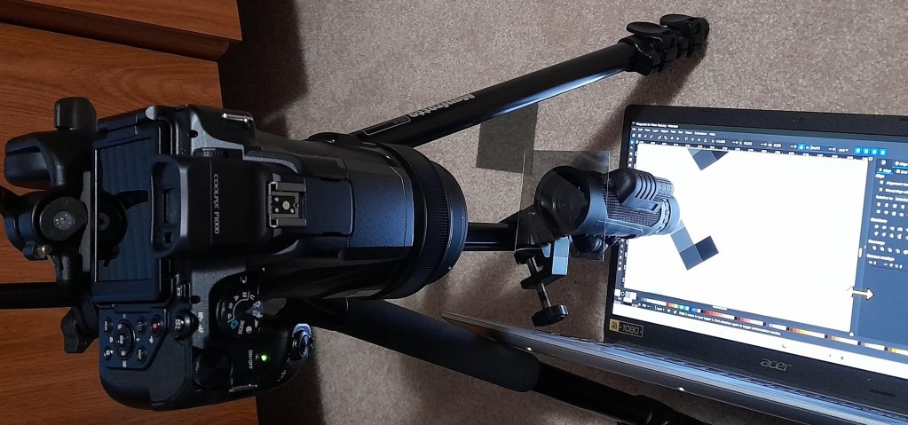
Images of the pupil as seen through the reversed monocular were then taken with the screen and monocular kept fixed but the orientation of the polarizer changed. This was facilitated by the use of a set of square targets that had been pre-rotated in 5-degree steps and placed linearly on the Inskscape canvas. Each target consisted of a series of small squares having different grayscale value, which would be used for a consistent set of reference tones. It was then simple to scroll from one image to the next and rotate the polarizer by hand so that it aligned with the next image, ensuring that the angles were accurate to within a degree or so.
Figure 3(a) shows a portion of the set of Inkscape grayscale targets. Figure 3(b) shows the setup for placing the polarizer over the target and photographing the result, with the camera settings kept identical as those used to record the images in the monocular.

After all of the images were assembled for analysis, the grayscale square which produced the most similar range of results as those for the monocular was used to estimate the change in electric field intensity for the prism images, according to Malus’ Law:

Figure 4 shows the measured values for both the prism-based images (“P”) and the reference images (“R”) along with the angle. By using this approach, at no point was it necessary to measure or estimate light intensities from the photographic images. Instead, each result was compared to a series of reference images in order to determine the nearest match in grayscale tone.

The results from the estimates were then compared to the expected change in electric field based on the calculated elliptical polarization output profile from the Python analysis. In Figure 5(a) we show this result, based on an input polarization which is vertical and parallel to the roof line as viewed through the reversed monocular. In 5(b) we show the estimated field from the photographic analysis versus the expected field strength, as a function of the orientation angle for the polarizing sheet relative to vertical. This expected field strength is obtained from taking the projection of one of the these elliptical polarizations onto an axis rotated by a given angle. The estimated results follow the expected trend.
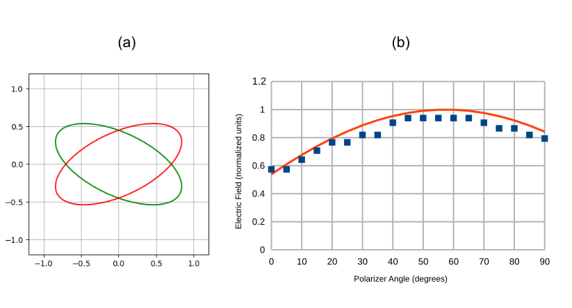
They key takeaways from this exercise are the following. First, the difference in intensity for an uncoated prism viewed between crossed and parallel polarizers does not yield a strikingly obvious change. Much care is needed if this is the only criteria used. Second, what is more apparent is the strong change in the gray tones between the two halves of the pupil when the polarization angle is around 60 degrees. Here, we will see the most contrast between the two sides, as the polarizer lies along the semimajor axis of one ellipse, which also results in near minimal transmission for the other. Hence the view will appear like black and white half circles with the greatest contrast. Third, carefully estimating the change in field strength via consistently captured images confirms the maximum transmission is near 60 degrees, in accord with the calculations.
Analysis of the Abbe-König prism design yields very similar results. The code below produces plots of the output polarization states for a number of user-configurable conditions. This is fairly verbose by intention, so that any tracing through the entire process and verifying all of the polarizations components is feasible, if desired. Note that the requirement, specified in the Zeiss paper, of having one polarizer along the roof line direction, is satisfied by setting phi to either 0 or 90 degrees. Intermediate angles will yield skewed, elliptically polarized results which are difficult to interpret. This explains why the Zeiss paper is adamant about the orientation.
Attached is a PDF of the Zeiss paper, including an English translation.
Geometries for the code are defined in Figure 6.

Python code to generate output polarization images.
# Polarization analysis for roof prisms - MJ Hurben 2024
import numpy as np
import matplotlib.pyplot as plt

# User-selectable settings
ng = 1.517  # Refractive index of prism glass
phi = 0  # Polarization angle in degrees relative to z-axis
phase_coating = False
prism_type = "SP"
prism_type = "AK"

def refl(In, N):
    Out = In - 2 * np.dot(In, N) * N
    return Out

def Svec(L, Lp):
    cross = np.cross(L, Lp)
    mag = np.linalg.norm(cross)
    return cross / mag

def C(PaP, SaP, Pb):
    A = np.dot(PaP, Pb)
    B = np.dot(SaP, Pb)
    return np.array([[A, B], [-B, A]])

def pMatrix(n, ang):
    dp = 2 * np.arctan(n * np.sqrt(n**2 * (np.sin(ang))**2 - 1) / np.cos(ang))
    ds = 2 * np.arctan(np.sqrt(n**2 * (np.sin(ang))**2 - 1) / (n * np.cos(ang)))
    d = np.abs(dp - ds)
    a = np.cos(d) + 1j * np.sin(d)
    return np.array([[a, 0], [0, 1]])

s2 = np.sqrt(2)
d2r = np.pi / 180  # Degrees to radians factor
om = 2 * np.pi  # Dummy frequency

# Construct the surface normal vectors
if prism_type == "SP":
    a = 45 * d2r
    b = 22.5 * d2r
    # Surface order: A,0,1,2,3,4
    NA = np.array([np.sin(a), 0, np.cos(a)])
    N0 = np.array([-np.sin(b), 0, -np.cos(b)])
    N1 = np.array([1, 0, 0])
    N4 = -NA
else:
    a = 30 * d2r
    b = 7.5 * d2r
    g = b + a  # Angle (gamma) of other non-roof surface is determined by alpha and beta
    # Surface order: 1,2,3,4
    N1 = np.array([np.sin(g), 0, -np.cos(g)])
    N4 = np.array([-np.sin(a), 0, -np.cos(a)])

# Roof surfaces are the same for both designs
N2 = (1/s2) * np.array([-np.sin(b), -1, np.cos(b)])
N3 = (1/s2) * np.array([-np.sin(b), 1, np.cos(b)])

# Input 2x1 polarization vector, zero phi angle corresponds to z direction
E0 = np.array([np.cos(phi * d2r), np.sin(phi * d2r)])

if prism_type == "SP":  # Incoming light is LA vector for SP prism
    # Left path k-vectors: unit vectors along propagation direction
    LA = np.array([-1, 0, 0])  # Input along negative x-direction
    LAp = refl(LA, NA)
    L0 = LAp
    L0p = refl(L0, N0)
    L1 = L0p
else:
    L1 = np.array([-1, 0, 0])  # Incoming light is L1 vector for AK prism

L1p = refl(L1, N1)
L2 = L1p

for path in range(0, 2):  # Two paths differ by order in which N2 and N3 are struck
    if path == 1:  # N2 first then N3
        L2p = refl(L2, N2)
        L3 = L2p
        L3p = refl(L3, N3)
    else:  # N3 then N2
        L2p = refl(L2, N3)
        L3 = L2p
        L3p = refl(L3, N2)

    L4 = L3p
    L4p = refl(L4, N4)

    # S vectors
    S1 = Svec(L1, L1p)
    S1p = S1
    S2 = Svec(L2, L2p)
    S2p = S2
    S3 = Svec(L3, L3p)
    S3p = S3
    S4 = Svec(L4, L4p)

    # P vectors
    P1 = np.cross(S1, L1)
    P1p = np.cross(S1p, L1p)
    P2 = np.cross(S2, L2)
    P2p = np.cross(S2p, L2p)
    P3 = np.cross(S3, L3)
    P3p = np.cross(S3p, L3p)
    P4 = np.cross(S4, L4)

    if prism_type == 'SP':  # Polarization vectors for Pechan prism only
        SA = Svec(LA, LAp)
        SAp = SA
        S0 = Svec(L0, L0p)
        S0p = S0
        PA = np.cross(SA, LA)
        PAp = np.cross(SAp, LAp)
        P0 = np.cross(S0, L0)
        P0p = np.cross(S0p, L0p)

        # Rotation Jones matrices for Pechan prism only
        CA0 = C(PAp, SAp, P0)
        C01 = C(P0p, S0p, P1)

    C12 = C(P1p, S1p, P2)
    C23 = C(P2p, S2p, P3)
    C34 = C(P3p, S3p, P4)

    # Phase shift Jones matrices
    ang1 = np.arccos(np.dot(L1, N1))
    ang2 = np.arccos(np.dot(L2, N2))  # Same applies to N3, by symmetry
    ang3 = np.arccos(np.dot(L4, N4))
    Po1 = pMatrix(ng, ang1)
    Po3 = pMatrix(ng, ang3)
    if phase_coating:
        Po2 = np.array([[-1, 0], [0, 1]])  # 180 degree shift convention
    else:
        Po2 = pMatrix(ng, ang2)
    if prism_type == 'SP':  # Additional TIR phase shift in Pechan prism
        angA = np.arccos(np.dot(LA, NA))
        PoA = pMatrix(ng, angA)
        if path == 1:
            EL = Po3 @ C34 @ Po2 @ C23 @ Po2 @ C12 @ Po1 @ C01 @ PoA @ CA0 @ E0
        else:
            ER = Po3 @ C34 @ Po2 @ C23 @ Po2 @ C12 @ Po1 @ C01 @ PoA @ CA0 @ E0
    else:  # AK with 2 less reflections
        if path == 1:
            EL = Po3 @ C34 @ Po2 @ C23 @ Po2 @ C12 @ Po1 @ E0
        else:
            ER = Po3 @ C34 @ Po2 @ C23 @ Po2 @ C12 @ Po1 @ E0

# Make the plot
EL_points = []
ER_points = []

for t in range(0, 102, 2):
    ELx = np.real(EL * (np.cos(om * t / 100) + 1j * np.sin(om * t / 100)))
    ERx = np.real(ER * (np.cos(om * t / 100) + 1j * np.sin(om * t / 100)))
    EL_points.append(ELx)
    ER_points.append(ERx)

EL_points = np.array(EL_points)
ER_points = np.array(ER_points)
plt.figure(figsize=(8, 8))
plt.plot(EL_points[:, 1], EL_points[:, 0], label='Left path')
plt.plot(ER_points[:, 1], ER_points[:, 0], label='Right path')
plt.xlim([-1.2, 1.2])
plt.ylim([-1.2, 1.2])
plt.grid(True)
plt.legend()
plt.title(f"Polarization Analysis for {prism_type} Prism")
plt.xlabel("Y-component")
plt.ylabel("Z-component")
plt.show()