
Introduction
It is well-known that the transmission of light through optical components such as lenses and prisms can be improved through the application of specialized dielectric coatings. We’ve come to take them for granted, and can easily forget that without them, the views through our instruments would be significantly dimmer. Any curious user of binoculars, cameras, and other equipment will, therefore, eventually find themselves wondering exactly why a series of thin optical layers can provide such a beneficial effect. At best it might seem like a free lunch, but from another perspective, it might even appear paradoxical. After all, every solid material that we place between a source of light and our eyes would seem to be just one more liability, not a benefit.
In a series of posts, we will explore this interesting topic, starting from the simplest cases and finishing up by considering some subtleties of multilayer designs. In doing all this, we will have a perfect opportunity to develop and use one of the most powerful, yet simple, analysis tools in optics, the transfer matrix method (TMM).
The TMM will be introduced in the following post. Here, we will begin with the simplest scenario of a single boundary between two optically different materials, such as air and glass. We will work out the conditions that the light must obey at the interface, and then determine how much light is reflected and transmitted when it meets this boundary in a perpendicular direction. We will then add a single layer coating and analyze its performance using a “brute force” approach which will suffice here, but not for more complicated scenarios. This will motivate our need to develop the TMM.
An Air to Glass Boundary Only
Consider a perfectly flat interface between regions having different refractive indices, and assume that light approaches in the first region where the index is  , the second medium has index
  , and that it meets the boundary in the normal (perpendicular) direction. (We chose these subscripts because “a” will correspond to air and “g” to glass.) Upon meeting the boundary, most of the light will be transmitted and the rest will be reflected. Our goal is to quantify exactly how much of the incident light goes each of these opposite directions.
We need to start with the boundary conditions for the electromagnetic waves involved. Since the wave is transverse and arrives in the perpendicular direction, the electric and magnetic fields must lie in the same plane as the boundary. The key expressions governing what happens at the boundary can be arrived at in several ways. One way is to enforce Maxwell’s equations for the waves at the interface. We will come back to such an approach in a later post. For now, though, we can simply note that the electric field and its slope must be continuous across the boundary. This accords with an intuitive constraint that will hold for any kind of wave that arrives at an interface at which there is a change in velocity.
Consider, for example, what would occur with two sections of string having different densities which are connected. When waves arrive at the boundary, the ends stay tied together (corresponding to a smooth change in amplitude), and there will be no discontinuously sharp kink at that point either (in other words, there will be a smoothly changing slope at all points, including at the connection).
Taking the spatial dependence of the field to be sinusoidal, depending on time and space, we will fix an incoming wave from the left to have an amplitude of 1.0, in arbitrary units, and assign the reflected and transmitted waves some amplitudes r and t, respectively. If we were to plot the electric field, we would have something like the animation shown in Figure 1, which just as easily would depict a less dense string on the left attached to a heaver one on the right.

For the mathematics, we have the total amplitudes on either side being equal, as well as the slopes, expressed as follows:


Note that these must hold for any value of the time  , and that the argument in the cosine for the reflected wave carries a negative sign to capture that it propagates in the opposite direction to the other waves. There are two different k (wavenumber) values to account for the different speeds in the two media.
At the boundary, where z=0, these two equations can be simplified by choosing values of  of zero or 90 degrees, respectively, which cause the trig functions to be eliminated, giving:


And solving for r, we have

Now we can use the simple relationship between frequency, wavenumber and velocity:

The frequency cannot change, so we have

With a similar simple expression for t:

Remember, the r and t values are magnitudes of the electric field. Since power goes as the square of the field, the energy reflection and transmission coefficients (aka reflectance and transmittance, respectively), which are what we really care about, will go as the squares of these, written as  and
and  . Where did the term
  come from? It is necessary to scale by this term to ensure energy conservation is satisfied, that is, that
  . We will use terms like transmittance and transmission interchangeably going forward, as we will always be referring to a value between 0 and 1 corresponding to the energy passing through a system. If we are discussing r and t, we will speak of field reflection coefficient and field transmission coefficient, respectively, each of which can vary between -1 and 1. The r and t are more useful in doing the calculations but it is always R and T that are our final metrics of interest.
Let’s now set  , so that we have the case of a vacuum (or approximately, air) as the first medium. We can now calculate and plot R and T as a function of the second index. This is shown in Figure 2.

When the glass index is equal to 1.0, we must have no reflection and full transmission, and that is what we find. As the index increases, the amount of reflection gets increasingly larger. Hence, higher index glass, which enables us to construct lenses with less curvature (a good thing) is going to produce more reflection (not so good). Reading off this plot, for an index of 1.5, we lose about 4% of the incoming light energy to reflection, passing 96% through the glass. This may seem like a lot of transmittance, but in a system with many elements, these losses will add up. Hence we are motivated to look for a coating that can reduce the reflection.
A Single Layer Coating
We will now consider how a single layer coating applied between the regions will affect the results. We will let the coating have an index  and a thickness
  . The situation is depicted in Figure 3.

If we did not think about this very hard, we might first expect that the presence of the coating is going to make the problem worse, because we now have reflections at both surfaces A and B instead of at only one surface. We shall see about that. Let us make a first guess or estimate for the final transmission T, and suggest that we simply multiply the t values at surfaces at A and B, and square the results, multiplying by the ratios  and
and  as well . This accounts for the cumulative loss in power after two boundaries are crossed. The value would be

We know from the plot in Figure 2 that the closer the two indices are, the larger the transmission. If we pick to be very close to the index for air, then we will get good transmission at A, but then we run into a problem at B. A similar problem happens if our coating has an index comparable to that of the glass. What we will want is something in between, and with some hindsight, that we will return to later, we will choose  .
.
Now setting to 1 and  , we will use
  , in which case at A we find the transmittance at each surface is T=0.9898, so the final transmittance according to our guess would be the product, or 97.97%. Recall that for the case of glass alone, the transmittance was 96%, so we have actually made a substantial improvement. Two gradual changes in refractive index result in less transmission loss than a single, abrupt change.
But this simple approach is wrong, because we are not looking at the full picture of what transpires at the two boundaries. Consider that after the light meets boundary A, anything reflected back to the left would seemingly be lost, but that the light reflected initially at surface B will have some portion reflected back (to the right) at A, which can then be transmitted as well. Some of that light will be reflected at B, of course, but then it too will get another reflection at A, and so on. This is shown graphically in Figure 4.

What should be clear is that there are an unlimited number of such reflection pairs that can contribute to the transmission of light, but that every time we add another cycle through the coating, we will have lost some of the energy. Hence, the total transmission is going to be a sum of terms that get progressively smaller.
At this point we need to remind ourselves that what we will be adding up are waves, and so we need to remember that they will superpose with one another, and that if there is any phase shift, we will see some amount of destructive interference. So let’s think about how to treat that for now by assuming that the light is monochromatic with wavelength  . Upon reflecting at B, assuming that
  holds, there must be an inversion of the wave, or a shift of 180 degrees. But upon reflecting back at A, there will be no phase shift because we have the case of going from a higher to a lower index.
As a reminder of why that is, Figure 5 shows an animation of a wave (blue) moving from a slower, high-index region on the left, into a faster region on the right (green), where the wavelength must be longer. In order to obey the boundary conditions here, the reflected wave (red) must be in phase; this allows the sum on the left (black) to smoothly connect at the boundary.

Now, back to the coating. If the thickness of the film corresponds to a quarter of the wavelength, all the phase changes will add to one wavelength, so perfect constructive interference will result, and the final transmission coefficient for the field can be written as

Or

Since both of the reflection coefficients must be less than one, we recognize that this is an infinite geometric series which converges to:

A lovely result! Let’s first note that the product in the numerator is:

The denominator works out to:

Now we see why we wanted  because the ratio then works out to:

So finally we have
 .
.
But what is the transmittance for light that has a different wavelength? A change in wavelength from nominal means that there will be some amount of destructive interference when we sum up all the waves, so that we will no longer have the simple geometric series above. Rather, each term that includes  must also be multiplied by a factor that accounts for a phase offset. Such terms are less than one, meaning that the result from the infinite sum will be less than it would be for the nominal wavelength. How much less? In Figure 6 we plot the transmission T versus wavelength, using results from a calculation method to be developed in the next post. Here we picked a nominal wavelength of 500 nm and show T over the full visible spectrum. The transmission falls off on either side, but note that even at the extremes, it is still a respectable 99%. Remember that with no coating, it would be 96% across this band.

It almost seems like we are getting something for nothing. Yes, we are harvesting the many reflections and using the quarter-wave thickness as a kind of “trap” to collect the light, but we might object that there are also an infinite number of reflections working against us. There is that first back reflection from A, and then some light reflected from B, and a little less that reflects at B, then A, then B again, and so on. The reason why this does not matter when the wavelength is nominal is because the initial reflection at A is inverted by 180 degrees, while all other reflective paths get no net phase shift. How is that? Well, the reflection at B causes a 180 degree shift, but in making two passes through a quarter-wave path, there is another shift of 180 degrees. Hence all the light reflected from B is out of phase with that reflected at A, so the interference is perfectly destructive. We will have a fully anti-reflection scenario for this one wavelength.
A practical question should be asked at this point. Given that our glass will have some specific refractive index that is an innate material property, will we be able to find a material for the coating whose index happens to be its square root (or sufficiently close to it)? The answer is almost always going to be no. Every coating material has some index, or maybe a small range of indices that depend on composition or deposition subtleties. And there are only so many materials amenable to deposition, which are durable, and so on. Any real-world solution is going to have to take into account that we cannot just ‘dial in’ any arbitrary index for a coating, even though we can do that for its thickness. More on how we will deal with this constraint in the next post.
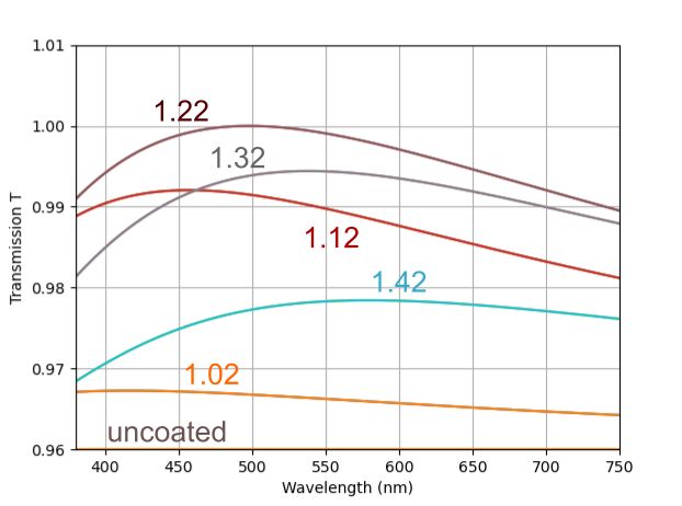
Using the same method that we’ll develop later, we can investigate just how much the transmittance through a single layer coating will be affected by changes to the coating’s index. Some results are shown in Figure 7, where we have kept the same thickness in each case. As can be seen, the situation with n=1.32 isn’t as good as n=1.22, but it still affords an overall big improvement over uncoated glass. (All of these scenarios, in fact, increase the overall transmittance, although they also introduce wavelength dependence, which we do not want.) A common coating material, cryolite, has an index of 1.35, and would offer some modest improvement compared to an uncoated glass.
Still, we’d like to do better. Not only do we want the maximum transmittance possible, we want to flatten this response: a perfect scenario would be a coating that provide perfect transmission across the entire visible range. This means we need to consider how multiple coating layers will perform—there really is no other way forward. We hope that with a judicious design using many different layers, we’ll be able to both increase and flatten the transmittance vs wavelength over the visual range using real materials. However, treating many layers will be difficult without some new tools, and that is what we will turn to in the next post, where we will look at multilayer performance and develop the transfer matrix method (TMM).
Main image credit: Michael Mommert, CC BY-SA 3.0 https://creativecommons.org/licenses/by-sa/3.0, via Wikimedia Commons