Anti-Reflection Coatings Part II: The Transfer Matrix Method

The Headache of Multiple Layers

In the previous post we calculated the effect of a single dielectric layer placed between air and glass, and showed that with a judicious selection of index and thickness, it would serve as an anti-reflection coating that would pass 100% of the light at a nominal wavelength, and at least 99% of the light throughout the rest of the visible spectrum. This “looked good on paper”, but because we cannot simply dial in the index of our coating, but rather have a limited set of materials to select from, we also saw that real world, single-layer solutions will be less than ideal.

If we hope to improve upon the transmittance across the visible spectrum, we’ll need to see if using additional layers with different indices might help. It is not immediately obvious that it will. After all, if one layer is tuned to pass 500 nm light, for example, and we add another layer that is nominal for 600 nm, won’t they affect one another, and each wreck the intended performance of the other? We will also have the questions of how to approach the design of a complex multilayer system and how to calculate its performance metrics. With the single layer, we were able to show that at least for the nominal wavelength, the transmission could be written out as an infinite geometric series which luckily had a well-known and simple expression. What will happen when we add more layers?

To get a feel for just how involved this can get, lets consider what happens when two layers with different indices lie between the air and the glass, and trace through just some of the paths that the light can take, starting with the simplest cases. Figure 1 shows this graphically. Most of the transmission will involve the “straight through” path at the top left, shown in green, which will have a total field transmission of t_At_Bt_C. Next are the cases with a single pair of reflections, which are shown in red. There are three ways for this to occur, and the transmission becomes more involved to write out. Finally, in blue we have all the possible ways in which four reflections can occur, of which there are eight. Of course, there are many more cases to consider having more reflections, but this is sufficient to make our point.

Figure 1. Schematic diagram showing the twelve simplest paths by which light can be transmitted through two layers. The direct path is shown in green. Cases with two reflections are in red, and those with four are in blue. In each case we have written out the net field transmission along that path.

What should be clear is that we are going to have a far more involved summation to deal with now; but keep in mind that this is only the case of two layers! Imagine the combinatorics for, say, a nine-layer system, and it will be obvious that the bookkeeping for all of these reflections is going to be a nightmare. What’s more, even when we had only a single layer, we had a clean expression only for the special case of the one wavelength for which the waves added with perfect constructive interference. For the other wavelengths, there are phase interference terms in the summation which will prevent writing out a simple result.

It appears that a multilayer coating does not present us with a trivial problem. Fortunately, there is an approach which makes the analysis straightforward, and which can be elegantly expressed with some fairly compact mathematics. Combining this with the immense computing power now available with even the least capable laptop, we will have a practical way to understand how multiple layer coatings will behave, and their design can be approached in a systematic way.

We note in passing that decades ago, the computational approach was not a feasible option, and that a number of approximation techniques had to be developed. These allowed designers to devise the nominal configuration of many dielectric layers in order to achieve some effect, such as broadband anti-reflection. These methods are not simple to derive, or intuitive to understand, so we will not discuss them here. See Macleod [1] for details.

We are now properly motivated to develop the mathematics needed for our computations, which is known as the transfer matrix method (TMM) for optical multilayers. It is a straightforward and elegant calculation method, and not hard to derive. It will allow us to bypass the headaches induced by the illustrations in Figure 1. Although it will not tell us how to design a coating, it will tell us exactly how any coating will perform, and so we’ll develop it first and then return to the practical question of how to devise a useful multilayer.

Transfer Matrix Method for Normal Incidence

We will begin by describing the basic idea behind the TMM in general terms, which involves two different kinds of 2 x 2 matrices that capture different effects. Then we will find explicit expressions for the elements of these matrices, using basic wave considerations. We will finish by working through some examples of coatings consisting of several layers, and then work to understand how a multilayer achieves its improvement over a single layer.

The approach of the TMM is to use a matrix to represent the connection between electromagnetic waves in two different locations which are separated by “something”, which causes them to be different. An interface between two different media is an example of a “something” that has such an effect. Another “something” is simply a finite space, which brings about a difference in phase. Let’s consider the case of a boundary first, as we already have some experience with this. The situation is shown in Figure 2.

Figure 2. Schematic for wave amplitudes and directions on either side of a boundary, which separates regions 1 and 2, having different refractive indices. The plus and minus signs indicate the wave propagation direction.

On the left, which we call location 1, we assume there is a wave with amplitude E₁⁺ moving to the right, and another with amplitude E₁^– moving to the left. Similarly for the other side. We will use two 2 x 1 column matrices to characterize the fields on either side, and express their relationship using a matrix $\mathcal{D}$ as follows:

$\begin{bmatrix} E_1^{+}\\E_1^{-}}\end{bmatrix} = \begin{bmatrix} D_{11} & D_{12} \\ D_{21} & D_{22} \end{bmatrix} \begin{bmatrix} E_2^{+}\\E_2^{-}}\end{bmatrix}$

We can work out the four values of this interface matrix by writing out the connections between the fields. We need to be careful about the coefficients, and will use subscripts to describe directions; the term “12” indicates light initially moving from region 1 towards 2, that is, to the right, and so on. We can see from Figure 2 that

$E_2^{+} = t_{12} E_1^{+} + r_{21} E_2^{-}$

$E_1^{-} = r_{12} E_1^{+} + t_{21} E_2^{-}$

Rearranging:

$E_1^{+} = 1/t_{12} (E_2^{+} - r_{21} E_2^{-})$

$E_1^{-} = r_{12}/t_{12} (E_2^{+} - r_{21} E_2^{-}) +t_{21} E_2^{-}$

Recall from the previous post that the reflection coefficient in going from region 1 to region 2 is:

$r_{12}=(n_1-n_2)/(n_1+n_2)$

And so $r_{21}=-r_{12}$ . For the transmission coefficient,

$t_{12}=2n_1/(n_1+n_2)$

So $t_{21}=t_{12}$ . When we combine all these, and make use of the fact that $R+T=1$ , we finally have the full interface matrix equation:

$\begin{bmatrix} E_1^{+}\\E_1^{-}}\end{bmatrix} = 1/t_{12} \begin{bmatrix} 1 & r_{12} \\ r_{12} & 1 \end{bmatrix} \begin{bmatrix} E_2^{+}\\E_2^{-}}\end{bmatrix}$

A very elegant result. Next we ask, how would the two electric field matrices be related if, instead of a boundary between them, they we separated by a space of width d and index n? This situation is depicted in Figure 3.

Figure 3. Schematic for wave amplitudes and directions on either side of space of width d and index n. In this case, the two regions share the same index, but are simply separated by space, which means that there will be a phase difference between the fields on either side.

We must consider this question because our stack of layers will consist not only of many interfaces, but of space between the interfaces. We will call the 2 x 2 matrix in this case the propagation matrix $\mathcal{P}$ , and write

$\begin{bmatrix} E_1^{+}\\E_1^{-}}\end{bmatrix} = \begin{bmatrix} P_{11} & P_{12} \\ P_{21} & P_{22} \end{bmatrix} \begin{bmatrix} E_2^{+}\\E_2^{-}}\end{bmatrix}$

Finding the coefficients here is even easier, because we know that the fields can be written as plane waves. That is

$E^{\pm} = E_0 e^{i(\omega \tau \pm kx)}$

So $E_2^{+} = E_1^{+} e^{ikd}$ and $E_2^{-} = E_1^{-}e^{-ikd}$ , and we note that the k values will be proportional to the index n. The matrix is then

$\begin{bmatrix} E_1^{+}\\E_1^{-}}\end{bmatrix} = \begin{bmatrix} e^{-ikd} & 0 \\ 0 & e^{ikd} \end{bmatrix} \begin{bmatrix} E_2^{+}\\E_2^{-}}\end{bmatrix}$

Now let’s consider how we will use this formalism to describe a simple case, namely, a system with two layers, as shown in Figure 4 below.

Figure 4. Schematic diagram for the TMM as applied to a two-layer coating, which consists of regions 2 and 3, between regions 1 (nominally air) and 4 (nominally glass).

Our goal is to connect the fields on the far left side, denoted with a subscript 1, with those on the far right, denoted with subscript 4. We can do this by starting at the right side and working back to the left. We know that the fields on either side of the rightmost boundary are related by $\mathcal{E}_{3R} = \mathcal{D}_{34} \mathcal{E}_4$ . Here the subscript “3R” denotes the field at the right side of region 3, which is connected to the field at the left side of region 3 according to

$\mathcal{E}_{3L} = \mathcal{P}_{3} \mathcal{E}_{3R}$

This field we can then relate across the next boundary on the left using an interface matrix, and so on. We need not track each of the electric field matrices, but can eliminate those within the structure and leave an expression relating the left and right sides, namely

$\mathcal{M} = \mathcal{D}_{12} \mathcal{P}_2 \mathcal{D}_{23} \mathcal{P}_3 \mathcal{D}_{34}$

Such that

$\begin{bmatrix} E_1^{+}\\E_1^{-}}\end{bmatrix} = \begin{bmatrix} M_{11} & M_{12} \\ M_{21} & M_{22} \end{bmatrix} \begin{bmatrix} E_4^{+}\\E_4^{-}}\end{bmatrix}$

Because any series of layers consist of nothing more than alternating interfaces (each accounted for by a $\mathcal{D}_{ij}$ matrix) and regions of propagation (accounted for with a $\mathcal{P}_i$ matrix), it means that any structure can be analyzed in this way. All of the multiple reflections and potential paths are taken care of in one fell swoop. We merely need to write out each matrix, do the multiplication, and read out the transmission and reflection coefficients, because the final matrix must effectively act like a single interface. That means that the reflection from the multilayer is then found from:

$r = M_{12} / M_{11}$

Because

$M_{11}=1/t$ and $M_{12}=r/t$

We now have a formalism that will allow us to calculate the transmission and reflection for any system of layers that we might wish to construct. Before we move on to multilayers, lets apply this method to the case of the single layer treated in the previous post.

The Single Layer Using TMM

With a single layer we have two interface matrices bracketing a single propagation matrix:

$\mathcal{M} = 1/{t_{12}t_{23}} \begin{bmatrix} 1 & r_{12} \\ r_{12} & 1 \end{bmatrix} \begin{bmatrix} e^{-ikd} & 0 \\ 0 & e^{ikd} \end{bmatrix} \begin{bmatrix} 1 & r_{23} \\ r_{23} & 1 \end{bmatrix}$

We need not work out every element in the final matrix because we know the final reflection coefficient, $r_f$ , involves just two matrix elements:

$r_f = M_{12}/M_{11}$

This gives

$r_f = (r_{12}e^{-ikd}+r_{23}e^{ikr}) /(e^{-ikd}+r_{12}r_{23}e^{ikr})$

If we select our layer to have an index that is the square root of the product of the air and glass indices, as we did in the previous post, then the two r values on the right side are the same. It is not difficult to show, from there, that final reflectance is then

$|r_f|^2=4r^2\cos^2(\Phi)/(\cos^2(\Phi)(1+r^2)^2+\sin^2(\Phi)(r^2-1)^2)$

where

$\Phi=2\pi n d/\lambda$

If the product of thickness and index is a quarter of a wavelength, then $\Phi=\pi/2$ and the final reflectance must be zero. For a more general expression, we can subtract the squared reflectance from 1.0 to give the transmittance versus wavelength, which reproduces the transmittance vs. wavelength plot (Figure 6 in the previous post).

The above expressions are tractable, if not very intuitive, but this is for the limited case of a single layer. To write out closed form expressions for multilayer films will result in far more complex expressions. There is no good reason to go that route. Instead, we can take the formalism that we developed above, in which we construct a series of individually simple matrices, and then multiply them together, and do all of the work computationally. At the bottom of this post a simple Python program, for transmittance versus wavelength for any set of up to nine layers placed between air and a glass substrate and perpendicular incidence, is included.

Exploring a 4-layer Multilayer

In terms of seeing exactly what a multilayer films can do, we have several approaches. We can look at existing multilayer designs in the literature in order to explore what has already been established. We can also do our own trial-and-error approach, in which we guess, check, modify, and repeat a process of setting up a series of layers and looking at the results. We will do a bit of both as we continue along. What we do not have the tools to do in this treatment is to start with our desired design metrics, for example, “transmittance >99% from 380 to 750 nm” and deduce exactly what the multilayer will look like. We recognize that this is a complex, multivariate optimization problem, like so many other engineering scenarios. Luckily, fast computation makes such tasks feasible.

Incidentally, if you don’t want to run the Python code below but still wish to “play” with some multilayer configurations (up to three layers) and see how the reflectance versus wavelength is affected, see https://andtherewaslight.github.io/multilayer/. The site owner, Claudio, also includes through a detailed derivation of the TMM. In the next post we will broaden our TMM treatment to be as comprehensive as his, by including oblique incidence.

As a first exploration of our TMM code, we can look to reproduce some published results, as summarized in the Macleod text referenced below [1]. Specifically, we consider a four-layer coating described on page 127 of that book. The indices, including air and glass, are arranged from left to right with values of 1, 1.38, 2.0, 1.9, 1.38, and 1.52. The thicknesses are specified in terms of the “optical thicknesses” at a reference wavelength, as is often done in the literature. The four optical thicknesses, relative to wavelength, are 0.25, 0.25, 0.25, and 0.5, and the reference wavelength is 510 nm. Each layer thickness is then given by multiplying the wavelength by relative thickness and dividing by that layer’s index. Hence, in nm, the approximate layer thicknesses are 92.4, 63.8, 67.1, and 184.8. The reflectance R, as plotted in Macleod, as well as the calculated transmittance T using the TMM Python code, are shown in Figure 5.

Figure 5. (a) Reflectance R vs. wavelength, as well as the coating design, from Macleod, page 127. (b) Calculated transmittance T vs. wavelength using the TMM Python code, showing good reproduction of these results, as T=1-R.

Why It Works

The curves in Figure 5 show us that a well-designed multilayer can give us a flatter spectral response than a single layer design. It isn’t ideal, but it is an improvement, and we note that this only uses four layers. We should trust our hunch that adding even more will allow us to tailor this curve further. Because four layers is still somewhat tractable, this is a good time to try to understand exactly why this combination of layers has broadened the transmission profile, because it isn’t obvious why it should.

The best way to begin is to consider the least convoluted reflection paths through the mulilayer. Figure 6 shows all of the possible ways in which a pair of reflections can occur in this structure. In each case, we include the total field transmittance t₀, and all of the reflection and additional transmission coefficients together, which make for the net field transmittance t for each path. We also list the relative phase shifts relative to light which simply transits the structure without any reflections. At each of the five interfaces, we mark with a blue dot the reflections for which the phase is shifted (that is, the amplitude gets inverted) due to movement from a lower to a higher index; it is critical to keep track of these inversions, which result in an additional factor of $\pi$ in the accumulated phase.

Figure 6. A four layer coating, with each layer designated by a number. The interfaces are designated by letters. The refractive indices are listed at the top. The straight-through path, together with the ten ways to get a pair of reflections, are shown, along with their net field transmittance and total relative accumulated phase shift. Blue dots indicate an inversion upon reflection.

Note that wavelength is going to enter into this via the phase terms, which are given by

$\Phi_i = 2\pi n_i d_i / \lambda$

The idea now is to take the initial term with no reflections, and all the field transmissions for the next ten cases, and treat this as our first approximation of the final answer. We know that the remaining terms will be smaller than these, because we have to multiply by at least two r factors for each additional set of reflections. Before we can add all theses terms, however, we must account for the phases, which we can do by setting the nominal phase to zero and then using a cosine to weight each term. That is, our approximate field transmission coefficient will be

$t_{approx} = t_0+\sum t_i \cos(\Phi_i)$

Finally, we will square this result and multiply by the ratio of initial to final index to get the approximate power transmittance T. We can also calculate each of the terms in the sum as a function of the wavelength. It is useful to look at each one of these terms individually and see how they combine. We will start with a few of them in Figure 7(a) below. Each curve is denoted by a pair of letters that indicate the two reflecting surfaces, along with the partial sum. In this plot we only look at the first four terms.

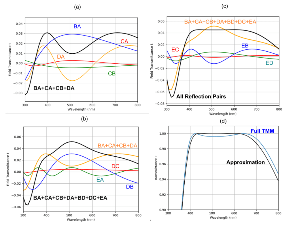
Figure 7. (a) Field transmission coefficients versus wavelength for four reflection pairs in a four layer multilayer, and their sum, in black. (b) The previous sum, now in orange, and the next three terms, leading to a sum of the first seven terms in black. (c) The previous sum, now in orange, and the next three terms, leading to a sum of all ten terms in black. (d) The resulting approximate power transmittance T based on this approximation (black) compared to the full TMM result (blue).

What we see is that the BA and DA reflections dominate, and the sum shown in the thick line allows BA to help reduce the large drop above 500 nm for the DA curve. In diagram (b), we redraw that result as the orange line, and then look at the next three terms, and take the full sum, which means the first seven terms, shown in black. Now we see that the DB curve helps bring up the central portion of the sum. In (c) we add the last three terms, which help to smooth out the wavelength dependence. Now we can add this curve to the flat transmittance t₀ and square it, which will give the approximation to T shown in black in diagram (d), with the full TMM result in blue. Our approximation is not too far off!

Anyone familiar with Fourier analysis can now see why multiple layers allow us to shape the spectral response—in this case into something relatively flat and broad. By having many layers to tune, we are effectively creating waveforms of field reflectance vs. wavelength, that will superpose just as we can use a collection of sine waves with different phases and wavelengths to construct an approximation to a periodic function. With more layers, we have more “components” to add and hence more freedom to shape the results.

Designing a 7-Layer Coating

With the code checked out, we can now try our hand at designing a multilayer film using real-world coating materials. In our example, we will try using two different materials, namely, magnesium fluoride, with an index of 1.38, and lead chloride, with an index of 2.3, alternating them to make a total of seven layers. This is another scenario which is discussed by Macleod [1], but instead of using his thickness recipe, which is optimized for performance from 400 to 700 nm, we will try finding a different design that provides transmittance of at least 99.5% over the wider bandwidth of 380 to 730 nm.

This is not hard to do if we have time. We simply sweep over a range of different layer thicknesses using a series of nested loops. For each scenario, we will calculate T for a number of wavelengths in our visible band, and note the lowest (worst) T value. Whenever we find a new scenario in which the minimum T value is better (higher) than any other, we will save that configuration as our best guess, and continue looking until we exhaust the space. Typically we will start with a coarse search, find and optimal setting, and then repeat with a fine sweep around that area. After sweeping though a parameter space, we will see if our best is good enough. If not, we can try a different range. And if that does not work, we can try adding more layers or incorporating other coating materials, and so on.

Figure 8 shows the results from this search for an acceptable recipe, in orange, together with the results for the nominal recipe described by Macleod (his Figure 4.50), in blue. Our new design sacrifices some of the transmittance from 400 to 700 nm, but it also extends the bandwidth over which T exceeds 0.995. The difference in thicknesses in nm is as follows: for Macleod, the values are 92.4, 33.5, 13.3, 51, 29.6, 14.2, and 179.2, while for the new recipe they are 94, 30, 16, 55, 30, 16, and 185.

Figure 8. Results for two similar 7-layer recipes, aiming for optimal transmittance between 400 and 700 nm (blue) or 380 and 730 nm (orange).

Obviously, the sky is the limit here, in terms of evaluating coating design. One merely needs computational power and time, as well as particular metric to minimize, or maximize. This can be applied to far more than anti-reflection coatings. Various calculations for phase-coating recipes needed for roof prisms, described in this post, used the same TMM approach and a similar optimization strategy.

In the next post, we will revise the TMM approach so that it can be used with light that arrives at an oblique incidence, instead of only in a perpendicular direction. This will lead to various color effects which may be evident when looking at coated lenses.

Python Code

# TMM for 9-layers - MJ Hurben Dec 2024 
import numpy as np
import matplotlib.pyplot as plt
d2r = np.pi / 180  # Degrees to radians factor
na=1 #Index of air
ng=1.52 # Index of glass

# n-Matrix: If less than 9 layers, use na for index of 'missing' layers
# d-Matrix values are in nm; initial air layers are arbitrary, final glass layer arbitrary

n=np.array([na,na,na,na,na,1.38,2.0,1.9,1.38,ng])
d=np.array([1,1,1,1,1,92.4,63.8,67.1,184.8,1000]) 

def PS(nva,dva,wl): # Phase Shift calculation

    def M(nA,nB): # Transfer matrix for interface
        r=(nA-nB)/(nA+nB)
        t=1+r
        d=1/t
        offd=r/t    
        m=np.array([[d,offd],[offd,d]]) 
        return m

    def P(L,n):  # Transfer matrix for propagation
        L=L*n*2*np.pi
        v=complex(np.cos(L),-np.sin(L))
        p=np.array([[v,0],[0,v.conjugate()]])
        return p
    
    W=M(nva[8],nva[9]) # Interface of last layer and glass
    for i in range(8,-1,-1):
        W=np.matmul(P(dva[i]/wl,nva[i]),W)
        if i>0:
            W=np.matmul(M(nva[i-1],nva[i]),W)
        else:
            W=np.matmul(M(na,nva[0]),W)  # Interface of glass and first layer 
        r=W[1,0]/W[0,0]     
    return r

wls=[] # Array of wavelengths
T=[] # Array of T values

for wl in range(380,751,2):
    r=PS(n,d,wl)
    wls.append(wl)
    T.append(1-abs(r)**2)
    
plt.grid(True)    
plt.plot(wls,T)
plt.xlim(380, 750)
plt.ylim(0.96,1.01)
plt.xlabel('Wavelength (nm)')
plt.ylabel('Transmittance T')

1 Macleod, H.A. (2021) “Thin-Film Optical Filters: Fifth Edition (Series in Optics and Optoelectronics),” 5th Edition, CRC Press.

Physics, Birding and Blindness

Michael Hurben, PhD